Normal Distribution (Bell Curve) - Definition and Examples | Marketing91

Hitesh Bhasin

marketing 91

Normal Distribution (Bell Curve) – Definition and Examples

July 10, 2021 By Hitesh Bhasin Tagged With: Management

Table of Contents

What is Bell Curve?

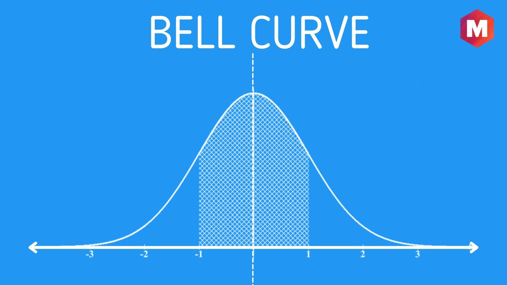
Definition: Bell curve is defined as a graphical depiction of a normal probability distribution whose standard deviations from the mean form a bell-shaped curve. A standard deviation is a measurement that helps quantify the variability of data dispersion, and the mean, on the other hand, is the average of all data points in the data set and is found on the highest point on the bell curve.

The bell curve, also known as Normal Distribution, refers to a type of probability distribution for a variable symmetric about the mean. It shows that data clustered around the mean occur more frequently than data far from the mean. Any graph that is used for depicting a normal distribution incorporates a symmetrical bell-shaped curve from where this term bell curve gets originated.

The bell curve has a wide application in the world of statistics. Financial analysts can use it to analyze security returns, while teachers can use a bell curve to compare test scores.

Psychologist Richard J. Herrnstein and political scientist Charles Murray in their book- The Bell Curve: Intelligence and Class Structure in American Life argued that human intelligence is substantially influenced by both inherited and environmental factors to explain the variations in intelligence in American society. For their book’s title, they used the bell-shaped normal distribution of intelligence quotient (IQ) scores in a population.

Understanding Bell Curve/Normal Distribution Concepts

The normal distribution or bell curve can be understood as a continuous probability distribution that is symmetrical on both sides of the mean in a way that the right side of the centre is the exact mirror image of the left side.

The area under the normal distribution is used for representing probability, plus the total area under the curve sums to one. This graph of probability density looks like a bell which gave it the name of the bell curve.

As a German mathematician, Carl Gauss first described the concept, normal distribution or bell curve is also known as Gaussian distribution.

Why is the Bell Curve important?

You can notice the bell-shaped curves as one of the common features of nature as well as psychology. It is the most crucial probability distribution in statistics because different sorts of continuous data in nature and psychology show the bell-shaped curve when they are being graphed and compiled.

For instance, if you randomly sample 50 people, you would see a bell curve for different continuous variables like IQ, weight, height, and blood pressure. For running different statistical tests that are more effective and powerful, psychologists need data to be normally distributed.

In case the data is not resembling a bell curve then researchers would opt for a less powerful type of statistical test named non-parametric statistics. The normal distribution process lets researchers determine the proportion of the values that come under a specific number of standard deviations from the mean.

Example of a Bell Curve

You can see a bell curve in the tests like the SAT and GRE in which greater numbers of students score the average (C), while on the other hand, the smaller numbers of students score a B or D. In addition, a smaller percentage of students score an F or an A.

This will create a bell-shaped distribution that will be symmetrical. In the bell curve, half of the test data will fall towards the left of the mean, while half of the data will fall towards the right. Different businesses use such tests in statistics, businesses, and government bodies such FDA for analyzing heights of people, blood pressure, measurement errors, IQ scores, points on a test, salaries, etc.

The empirical rule suggests what percentage of the data will fall within a specific number of standard deviations from the mean:

68% of the data will fall in one standard deviation of the mean
95% of the data will fall within two standard deviations of the mean
99.7% of the data will fall within three standard deviations of the mean

The standard deviation is used for controlling the spread of the distribution. When a smaller standard deviation occurs then it indicates that the data is tightly clustered around the mean which will result in a taller normal distribution. While if a larger standard deviation occurs then it will indicate that the data is spread out around the mean which will result in a flatter and wider normal distribution.

Properties of Bell Curve

All forms of bell curves share the following characteristics.

1. It is Symmetric

The bell curve has a perfectly symmetrical shape. The curve can be divided in the middle to produce two halves of equal size.

2. Equal Mean, Median, and Mode

The middle point of the bell shape curve refers to the highest frequency, which indicates that it possesses the most observations of the variable. All these three measures fall on the mid-point of the bell curve.

3. Kurtosis and Skewness

Kurtosis and skewness are coefficients that highlight how different a particular distribution is from a bell curve. While skewness measures the symmetry of the bell curve, kurtosis measures the thickness of the tail ends compared to the tales of a bell curve.

4. The Empirical Rule

When the data is usually distributed, there is a constant proportion of the distance between the mean of the data and a specific number of standard deviations from the mean. For instance, 95% of all cases fall within the range of +/- two standard deviations from the mean.

Importance of Bell Curve/Normal Distributions

1. Many Variables are Approximately Distributed Normally

Many educational and psychological variables often approximate a normal distribution. Measures such as reading ability, test scores, and job satisfaction are among the many variables that approximate a normal distribution.

2. Convenient to Work With

Mathematical statisticians find the bell shape curve easy to work with. This implies that several statistical tests can be derived from a normal distribution. These tests work successfully even if the variables approximate a normal distribution and are not exactly normally distributed.

3. Hypothesis Testing

Several statical hypothesis tests often assume that the data follows a normal distribution. It allows statisticians to decide whether they should accept or reject the null hypothesis.

4. Relevance in Regression Models

The normality assumption is followed by both linear as well as non-linear regression models. According to the normality assumption, the residuals in a regression model follow a normal distribution.

5. Relevance in the Central Limit Theorem

According to the central limit theorem, with an increase in the sample size, the sampling distribution of the mean tends to follow a normal distribution.

Limitations of the Bell Curve in the Practical World

1. Not Feasible for Small Sample Sizes

The bell curve is accurate at differentiating between data points when the sample size is large. This is not surprising; almost all statistical methods provide a more precise measure when the sample size increases. However, in small sample size, using a normal distribution can lead to several errors while making statistical inferences.

2. Datasets Are Not Perfectly Normal

In reality, a dataset is not perfectly regular. This can be due to several reasons. Sometimes there is a lack of symmetry or skewness. Other times the distribution might have excess kurtosis with fat tails. This makes tail events more probable than the predictions of the normal distribution.

Wrap Up!

The benefits provided to statisticians by using the bell curve outweigh the two significant problems caused by it. It has a wide range of applications in statistics, which has helped in conducting several hypothesis tests and drawing statistical inferences.

Due to the immense number of variables that exhibit normal behavior, the bell-shaped curve has become a commonly used tool in inferential statistics. All in all, the bell curve can be understood as a statistical concept relating to the normal distribution.

Interpretation of a bell curve suggests that the points that are nearest to the center of the bell curve will be those which have more chances to occur, while the point that is closest to the left and right edges are considered as the outliers. This way, a bell curve is used across multiple disciplines such as finance, economics, natural sciences, social science, etc.

ORIGINAL Article